1. Purpose and Application:

    The deep neural network is currently the most powerful machine learning technique. However, it requires high computation effort, especially in MAC (multiply-accumulate) operations, which is not applicable to smaller devices with power constraints.

    Stochastic computation requires extremely low cost and power consumption compared to conventional fixed-point arithmetic. However, it comes with random errors and longer latency. In this project, our team is trying to find out a more powerful stochastic computation method to shorten the latency while not sacrificing the accuracy.

    Deep neural network (DNN) is a machine learning technology that has become popular in recent years, which is very powerful. However, it also requires considerable computing resources and memory. It is time-consuming to train or test by using CPU alone on PC,  so it is often necessary to put the data on other hardware for accelerating. The most commonly used accelerator is the GPU.

The main advantage of the GPU lies in its powerful parallel computing capabilities. However, the power consumption required is also very large, this will be difficult to load for normal mobile devices. At this time, FPGA or ASIC will have its advantages. Because FPGA  can control its hardware usage more flexible,  both memory and logic gates can be customized, also, the overall resources can be used more efficiently, and the power consumption is lower. 

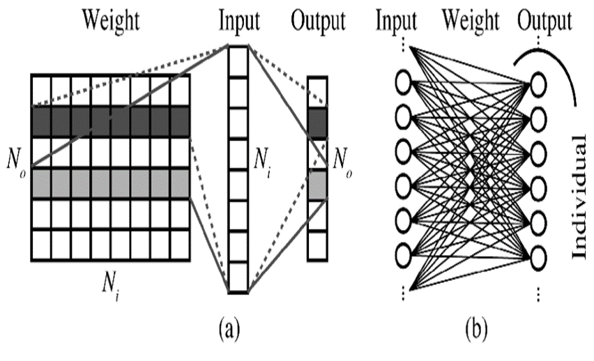
DNN is composed of multiple hidden layers. As shown in figure (b) below, each layer will have a different number of neurons (the number is called hidden dimension).  For an input vector, each element is multiplied by a set of weights and added to the neuron. Finally, the value of this layer is passed to an activation function (sigmoid、tanh、relu are often used) as the input vector of the next layer.

We can think of the above process as a matrix-vector multiplication, as shown in figure (a) below. All the connected weight can be expressed as a weight matrix W, and input can represent a unique vector x. Then, the output y is passed to the next layer through the activation function. Thus, the main calculation of the DNN lies in the matrix-vector multiplication, which is the part that we want to implement with FPGA.

2. Target users:

• Companies trying to add AI features (deep learning models) to their products with power constraints.
• Developer interested in deep learning and its computation method.

3. Features:

In this project, our team will construct a neural network acceleration block on Altera FPGA with following features.

• Support the operations in fully connected layers and convolution layers, including matrix-vector multiplication and several activation functions (sigmoid, tanh, relu).
• Users can change the length of stochastic bit-stream arbitrarily depending on the trade-off between accuracy and latency.
• Three computation mode(more details in Block diagram section):
  • Conventional fixed-point arithmetic: using an embedded multiplier or DSP.
  • Stochastic arithmetic: using our custom module.
  • Hybrid method: combine the above-mentioned two arithmetic to boost the overall computation performance.

1. FPGA和ARM CPU的組合，同時兼具了軟體開發的優點靈活性，以及客製化硬體的高效率。同時板子上還提供了許多外接插口，可以與其他開發版組合來達到更多功能。
2. FPGA的改動相對容易，適應性非常強，可以根據不同的需求設計其架構，達到高效能的表現。
3. 在我們的專題中，我們使用FPGA完成了一高效率的矩陣乘法計算器，並利用嵌入ARM CPU去讀取資料並與各模組進行資料間的溝通與傳輸。

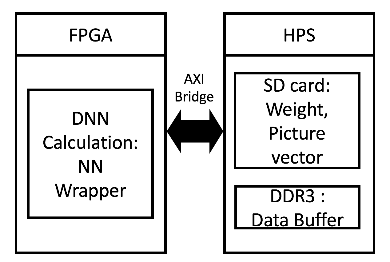
Hard/Software Partition

我們會將整個架構分成2個主要部分：

1. Hardware：Stochastic computation based的矩陣-向量乘法器 
2. Software：處理資料的 I/O以及SDRAM之存取，以CPU(ARM Processor執行)

We split the design into two parts :

1. Hardware：Matrix-Vector Multiplier based on a Stochastic computation
2. Software：Using CPU(ARM processor) to deal with the I/O data and access the SDRAM data.

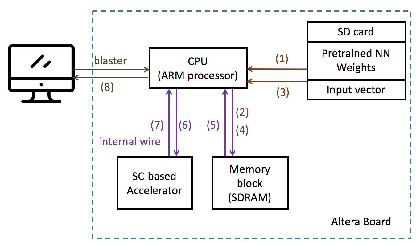
工作流程 Workflow

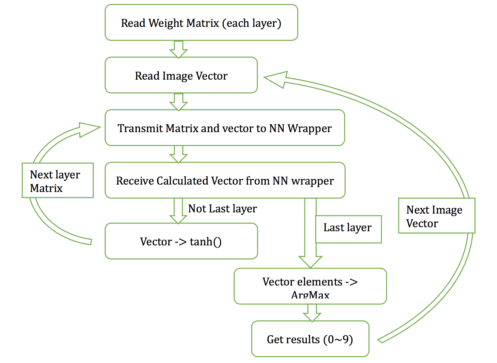
整體的工作流程如下圖所示，以下將進行簡單的步驟說明。

The overall workflow is as shown in the figure below. The following steps will be explained briefly.

1. 我們會先用電腦train好一個DNN，並將模型的參數(每一層layer的Weights)存在SDcard並傳入FPGA
2. CPU將接收到的weight matrix W寫進SDRAM中
3. 電腦將一筆input vector x傳入(在MNIST上就是一張圖片，28*28維)
4. CPU將接收到的x寫進SDRAM中
5. CPU自SDRAM讀取W的一個column以及目前的x
6. CPU將資料傳入我們的IP 矩陣-向量乘法器中
7. CPU接收矩陣-向量乘法器所計算出的結果，重複進行(5)、(6)直到這層layer計算結束，再進行下一層layer的計算。
8. CPU將最終的結果傳回電腦中。電腦接收後可以在傳入另一組x，重複(2)~(8)之步驟。

1. We will first use a computer to train a DNN and store the model parameters (the thickness of each layer) in the SDcard and pass it to the FPGA.
2. We will first use a computer to train a DNN and store the model parameters (the thickness of each layer) in the SDcard and pass it to the FPGA.
3. The computer passes in an input vector x (a picture on MNIST, 28*28 dimensions).
4. CPU writes received x into SDRAM.
5. CPU reads a column of W from SDRAM and the current x
6. CPU passes data into our IP matrix-vector multiplier.
7. The CPU receives the result calculated by the matrix-vector multiplier and repeats (5) and (6) until the layer calculation is completed and then performs the calculation of the next layer.
8. The CPU sends the final result back to the computer. The computer can receive another group x after receiving and repeat steps (2)~(8).

Stochastic Computation (SC) Introduction：

SC的概念相當簡單，對任何一個介在0~1之間的數字，我們可以將其轉換為一0、1組成的random bit stream，其中1出現的機率便是其數值大小。如圖下圖所示，假設現在我們有兩個數P1、P2並將其轉換為2個沒有correlation的bit stream，將這2個通過AND gate得到bit stream，對其我們用累加counter去計算1出現的機率便是P1*P2的結果，對於負數以及其他四則運算SC有都有其相應的算法。簡單的說，SC可以將龐大且複雜的乘法器架構轉換成一個AND gate，省下許多的Logic elements，因此可以大量的進行平行化的運算。

The concept of the SC is quite simple. For any number between 0 and 1, we can convert it into a random bit stream of 0, 1, where the probability of 1 is its magnitude. As shown in the figure below, suppose we now have two numbers P1 and P2 and convert them into two bitstreams without correlation. The result of P1*P2 is the probability of 1 accumulated by the counter from the bit stream which is the AND of the two streams P1, P2. There are corresponding algorithms for negative numbers and other four arithmetic SCs. Simply put, SC can convert a huge and complex multiplier architecture into an AND gate, saving a lot of Logic elements, so it can do a lot of parallel operations.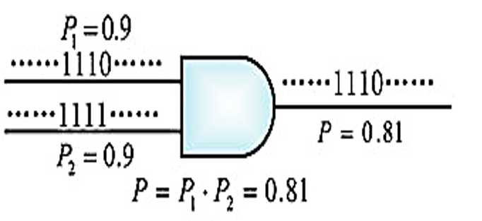

SC的優缺點大可以整理如下：

The advantages and disadvantages of SC can be summarized as follows:

SC Matric-Vector Multiplier

這部分的乘法器架構，我們主要會參考DAC2017的一篇論文：

This part of the multiplier architecture, we mainly refer to a DAC2017 paper:

Sim, Hyeonuk, and Jongeun Lee. "A New Stochastic Computing Multiplier with Application to Deep Convolutional Neural Networks." Proceedings of the 54th Annual Design Automation Conference 2017. ACM, 2017.

並進行改良與實作，其主要架構如下圖所示(圖片擷取自該篇論文，並有稍作修改)

And to carry out improvement and implementation, the main structure is shown in the figure below (the picture was taken from this paper, with some minor modifications)

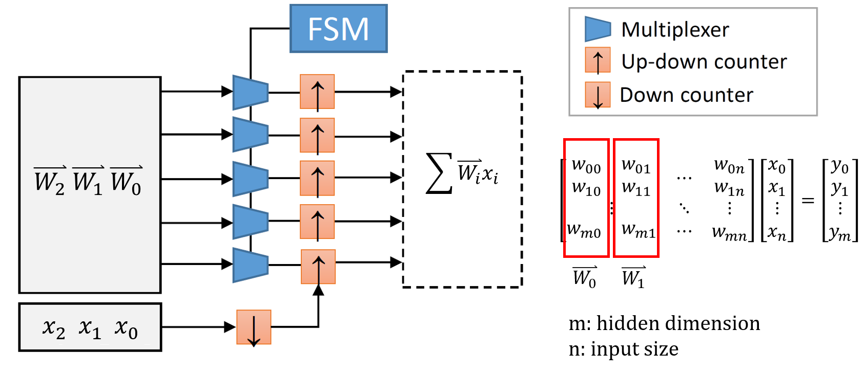
選用此架構的原因主要有二：

There are two main reasons for choosing this architecture:

1. 其中所提出的random bit stream產生並非隨機，而是用一種決定性(deterministic)的算法，因此可以以效降低一般SC算法中的誤差。
2. 具有良好的平行化架構，並可以有效的重複利用硬體，達到高效的運算。

1. The proposed random bit stream generation is not random but uses a deterministic algorithm, so it can effectively reduce the error in the general SC algorithm.
2. Has a good parallel architecture, and can effectively reuse hardware to achieve efficient computing.

NNWrapper：

將上述架構在包成了一個NN_Wrapper的ip，負責和ARM CPU藉由AXI bridge進行資料溝通。其state graph如圖[7]所示。

The above architecture is packaged into an IP named NN_Wrapper responsible for communicating with the ARM CPU through the AXI bridge. Its state graph is shown in Figure [7].

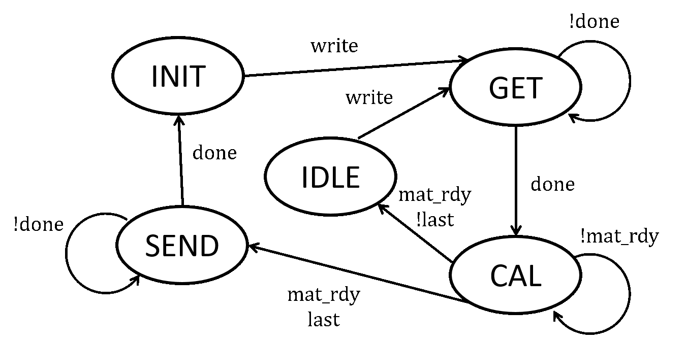
圖[7] NN_Wrapper state graph

State簡介：

1.INIT:

初始化，會將Mat_Mul中的up-down counter歸零，並將其中的所有buffer或reg清空。

2.GET：

讀取CPU所傳入的資料，每一次會將一個W的一個column加上所對應的input vector的element傳入，每個數值皆用8 bit表示。由於目前只使用32bit的AXI bridge，因此會分多次傳入。

3. CAL：

將收集完資料後將其傳入矩陣-向量乘法器Mat_Mul中，等待其計算完成(mat_rdy=1)。

4. IDLE：

表示這次傳入的資料不是最後一個column，等待CPU將下一個column及對應的input vector的element傳入。

5. SEND：

表示這次傳入的資料已經是最後一筆資料，會將結果傳回給Avalon master，由於每次一樣只能傳輸32 bit，因此會分多次傳出，每個值會以32 bit表示，傳輸完成後回到INIT。

 Introduction of state:

1.INIT:

Initialization. will reset the up-down counter in Mat_Mul to zero and empty all buffers or regs.

2.GET:

Read the data input from the CPU. Each time the element of the corresponding input vector is added to a column of W, and each value is represented by 8 bits. Since the 32-bit AXI bridge is used, it will transmit in multiple times.

3.CAL:

After the data is collected, it is passed to the matrix-vector multiplier Mat_Mul, and wait for the computation to be complete (mat_rdy=1).

4.IDLE:

Indicates that the incoming data is not the last column, waiting for the CPU to pass in the next column and the element of the corresponding input vector.

5.SEND:

Indicates that the incoming data is already the last data, the result will be passed back to the Avalon master. Since only 32 bits can be transmitted each time, it will be transmitted multiple times. Each value will be represented by 32 bits and it will return to INIT state after the transmission completed.

Performance Parameters

首先，先介紹一下我們所進行實驗的神經網路架構：

First of all, first introduce the neural network architecture we are experimenting with:

一、DNN model架構 (structure)：

我們以MNIST作為實驗的dataset，並使用tensorflow疊了一個簡單DNN，每層都不加bias，activation function為tanh，最後一層為softmax，並minimize其cross entropy，使用的optimizer為Adam(lr=0.001)，各層的dimension為784 → 50 → 50 → 50 → 10。

We use MNIST as the experimental dataset and use tensorflow to stack a simple DNN. Each layer does not add bias, the activation function is tanh, the last layer is softmax, and it minimizes its cross entropy. The used optimizer is Adam (lr=0.001). The dimension of each floor is 784 → 50 → 50 → 50 → 10.

二、數值限制 (Numerical limit)：

為了讓這個DNN model更容易在我們的硬體架構中執行，我對Weights及MNIST圖片的每個pixel值進行了以下限制：

In order to make this DNN model easier to implement in our hardware architecture, I made the following restrictions on each pixel value of the Weights and MNIST images:

1. 1. 每個數值限制在-1~1之間，因為這是SC能處理的數字範圍。當然沒有這道限制的話也是有有相應的解決辦法，就是在送進去之前先將其scale到-1~1之間，等計算完後再rescale，不過這部分會需要額外的計算時間，而且可能會降低我們SC架構的正確率。Each value is limited to -1 to 1, because this is the number range that the SC can handle. Of course, if there is no such restriction, there is a corresponding solution. It is to scale it to -1~1 before sending it in. After the calculation, it will be rescaled. However, this part may require extra calculation time, and it may Will reduce the accuracy of our SC architecture.
   2. 將數值的精確度限制在2^-7，表示數值只會是Limit the numerical accuracy to 2^-7, indicating that the value will only be

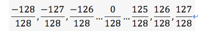
         256個值的其中一種。

         0One of 256 values.

SC error analysis

一、單一乘法器 Single multiplier

在參考資料[4]中，提到在傳統的SC乘法中，當2個數字很接近0的時候得到的誤差會較大，其error surface如圖[22](a)所示(x、y軸表示相乘的兩數，z軸表示誤差)，我們對使用的架構做了同樣的分析以同樣的的形式畫了一張，如圖[22](b)。

In reference [4], it is mentioned that in traditional SC multiplication, when two numbers are close to zero, the error obtained is larger, and its error surface is shown in [22](a) (x, y). The axis represents the multiplicative number, and the z-axis represents the error. We performed the same analysis on the architecture used and drew the same form, as shown in Fig. [22](b).

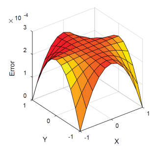
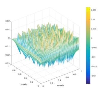
        圖[22] (a) Conventional SC (1024-bit stream)   (b)our SC(128-bit stream)

可以發現到兩者的error分布是不太一樣的，我們的error並沒有在接近0的時候明顯較高，反倒是成一種規律的鋸齒狀分布。

It can be found that the error distribution of the two is not the same. Our error is not significantly higher when it is close to 0, but instead it is a regular jagged distribution.

二、整體(以上述DNN在FPGA上實測) Overall (measured on the FPGA with the above DNN)

最後訓練出來的testing正確率為96.76%，對MNIST來說不算太好，不過這並不是本次實驗的重點。在這部分我們主要是要測試在FPGA版上每輸入一筆input是否能得到和在電腦上用tensorflow跑出的結果一致。使用之bit stream長度為128。實驗了10,000張圖片，結果記錄於表[4]。

The final training test rate of 96.76% is not too good for MNIST, but this is not the focus of this experiment. In this part, we mainly want to test whether the input of a single input in the FPGA version can be consistent with the result of running out of tensorflow on the computer. The length of the used bit stream is 128. 10,000 pictures were tested and the results are recorded in Table [4].

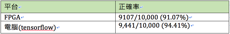
表[4] 實測結果 Table [4] Measured results

Latency分析 (Analysis)：

一、理論值 First, the theoretical value

1. 傳輸時間 Transmission time

我們使用的clock頻率為50MHz，因此一個clock cycle(c.c.)為20ns。以下為各步驟所需時間，算法中有些部分與我們實作細節有關。

The clock frequency we use is 50MHz, so a clock cycle (c.c.) is 20ns. The following is the time required for each step. Some parts of the algorithm are related to our actual details.

傳送weight及input vector ( Send weight and input vector )

784+50+50+50×13=12142 (c.c.) 

讀取ip計算結果 ( Read ip calculation result )

784+50+50+50×50+51=94334 (c.c.)

共計106476個c.c.，為2.13ms。 ( A total of 106,476 c.c., which is 2.13 ms. )

     2. 矩陣乘法計算時間 ( Matrix multiplication calculation time )

在前面所介紹的硬體架構中(參見圖[4、6])，我們會把down counter初始化為x的大小，因此由x的大小可以知道每次需要多少個c.c.，下圖為每層layer之input vector大小(絕對值)分布

In the hardware architecture introduced earlier (see Figure [4, 6]), we will initialize the down counter to the size of x, so the size of x can be used to know how many ccs are needed at a time. The following figure shows each layer. The input vector size (absolute value) distribution

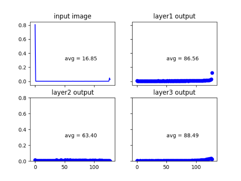
因此我們可以計算出平均耗時為( So we can calculate the average time )

784×16.85+50×86.56+63.40+88.49=25132.9 c.c.

為0.50ms。

因此我們可以得出，在不考慮CPU中其他operation造成的耗時的情況下，平均latency的理論值為2.63ms。

Therefore, we can conclude that the average value of latency is 2.63 ms without taking into account the time consumed by other operations in the CPU.

二、實驗值 ( Experimental value )

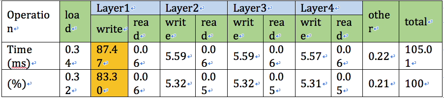
      我們以c語言的標準函式庫中time.h進行量測，結果整理於下表

We measure in time.h in the standard language library of c language. The results are summarized in the table below

每個operation所代表的函意：(The correspondence represented by each operation: )

1. laod: 將圖片自SD card讀入memory
2. write: 將該層layer的weights和input vector以AXI bridge傳入NN_Wrapper
3. read: 將該層layer的計算結果以AXI bridge讀入memory，也包含了矩陣乘法的計算時間
4. other: CPU需要處理的其他工作，像是tanh、argmax等。

1. Laod: Reading pictures from SD card into memory
2. Write: Pass the layer's weights and input vector into the NN_Wrapper as AXI bridge
3. Read: The layer's calculation result is read into the memory as an AXI bridge. It also contains the calculation time of the matrix multiplication.
4. Other: Other tasks that the CPU needs to handle, such as tanh, argmax, etc.

由上表可以發現到write占了絕大多數的時間(共計99.25%)，尤其是第一層layer，而且花掉的時間遠大於理論值。目前還不確定是什麼緣故，有可能是我們在從memory中讀取數據時就花掉了一定量的時間。整體來講，跑完一張MNIST圖要需要105ms，表示1秒大概只能處理9~10張圖片，效率上是非常低的，目前能想到幾個降低latency的方法就是增加AXI bridge的寬度，以縮短傳輸時間，以及修改ARM執行的C code，使其更有效率，不過我們並沒有時間進行這部分的嘗試。

From the above table, it can be found that write accounted for most of the time (a total of 99.25%), especially the first layer, and it took much longer than the theoretical value. It's not yet clear what the reason is, and it may be that we spend a certain amount of time reading data from memory. Overall speaking, it takes 105ms to complete a MNIST chart, which means that one second can only process 9~10 images. The efficiency is very low. At present, we can think of several ways to reduce the latency by increasing the width of the AXI bridge. In order to shorten the transmission time and modify the ARM code to make it more efficient, we do not have time to try this part.

Software flow

Future work

捲積層(Convolution layer)：
捲積神經網路(CNN)是面前在處理影像上表現最好的模型架構，它的計算方法與先前提到的DNN的fully-connected layer有點不同，會將每個filter(kernel)的weight點對點的乘上對應的input最為output，並在將filter移動後再進行一次這樣的計算，以4x4的input，以及2x2的filter為例，在不考慮padding的情況下，其過程如下圖所示。

A convolutional neural network (CNN) is the best model architecture for processing images. Its calculation method is slightly different from that of the previously mentioned DNN's fully-connected layer. It will weight each filter (kernel) point-to-point. Multiply the corresponding input with the most output, and perform a calculation after moving the filter. Take the 4x4 input and the 2x2 filter as examples. The process is as follows without considering padding.

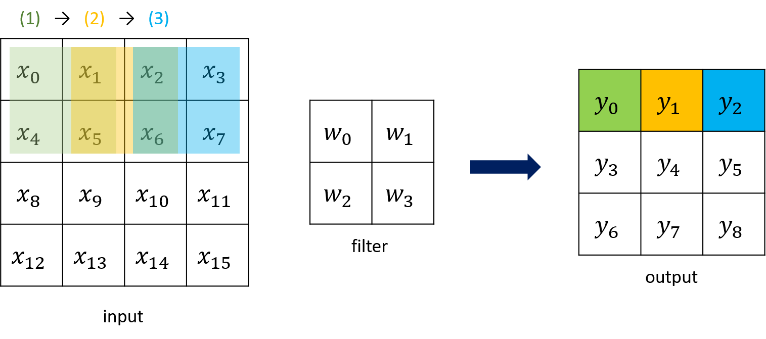
若是我們將上面的過程整理後，可以發現到其實2D convolution也可以化簡成一矩陣-向量乘法，如下圖所示。

If we organize the above process, we can see that in fact, 2D convolution can also be reduced to a matrix-vector multiplication, as shown in the following figure.

因此這部分的計算也可以使用我們的矩陣-向量乘法器進行運算，只需要將提取W、x以及將其送入custom IP的過程即可。

So this part of the calculation can also use our matrix-vector multiplier to perform the operation, just to extract the W, x and send it to the custom IP process.

整合DE10內置乘法器與DSP：(Integrate DE10 built-in multiplier and DSP)
SC雖有邏輯閘使用較少的主要優點，但依舊存在著許多缺點，加上板子上本來就含有embedded multiplier，不使用也是浪費，因此我們可以將一些精確度需求較高的計算(如捲積層)移到內置的乘法器上進行計算。如此一來不但可以增加整體的正確率，也可以提高throughput，更加完整的利用了FPGA板的硬體資源。

Although SC has the main advantage of using fewer logic gates, there are still many shortcomings. Plus, embedded multipliers are already included on the board. It is also wasteful to not use them. Therefore, we can use some calculations with higher precision (such as convolutional layers). ) Move to the built-in multiplier for calculation. This can not only increase the overall accuracy rate but also improve throughput, making full use of the hardware resources of the FPGA board.